Logistic Regression

Logistic regression is a supervised machine learning algorithm used in classification tasks where a target variable $y$ may take $K$ possible values, and we are interested in labeling an observation $\mathbf{x}$ composed of $N$ features/predictors. In particular, logistic regression is used in binary classification tasks, i.e., cases where $K=2$. However, by combining multiple logistic regression classifiers, it is possible to extend their use to multinomial cases, i.e., scenarios where $K>2$. The idea behind logistic regression is to estimate the probability a posteriori of $y$ given $\mathbf{x}$, and then assign an estimated class to $\mathbf{x}$ according to a decision rule based on the estimation.

Binary Classification

The target variable can only take two possibles values, e.g., “yes/no”, “win/lose”, “apple/orange”, “woman/man”. We usually use 0 and 1 to numerically represent these values, i.e., $y \in \left\{0, 1\right\}$. This way, in each respective scenario, $y=1$ may represent “yes”, “win”, “apple” or “woman”, while $y=0$ be associated to “no”, “lose”, “orange” or “man”. We can also assign the labels in the opposite order, this actually has no impact on the performance of logistic regression.

Sigmoid Function

One of the main components of logistic regression is the sigmoid function $\sigma: \mathbb{R}\to (0, 1)$, defined as

According to Eq. (\ref{sigmoid}), $\sigma(z)$ always lays between 0 and 1. In particular, since $e^0 = 1$, then $\sigma(0) = 1/2$. For large values of $z$, the term $e^z$ becomes a large positive number, and $\sigma(z)$ tends to $1$. On the other hand, when $z$ takes large negative values, $e^z$ approaches $0$, and thus $\sigma(z)$ is close to $0$. The fact that the image of the sigmoid function is constrained to the interval $(0, 1)$ allows to use this function to express the probability of an event.

In addition, we have

which means that $1 - \sigma(z)$ is a mirrored copy of $\sigma(z)$.

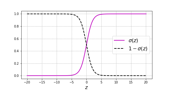
Sigmoid function $\sigma(z)$ and $1 - \sigma(z)$.

At the same time, it is trivial to show that

Finally, we can see that

Since $\sigma(z)$ and $1- \sigma(z)$ are always positive, so is $\sigma’(z)$, and thus $\sigma(z)$ is a monotonically increasing function. While the maximum of $\sigma’(z)$ is placed in $z=0$, as the module of $z$ increases, $\sigma’(z)$ approaches zero in a symmetrical way since $\sigma’(z) = \sigma’(-z)$, i.e. $\sigma’(z)$ is an even function.

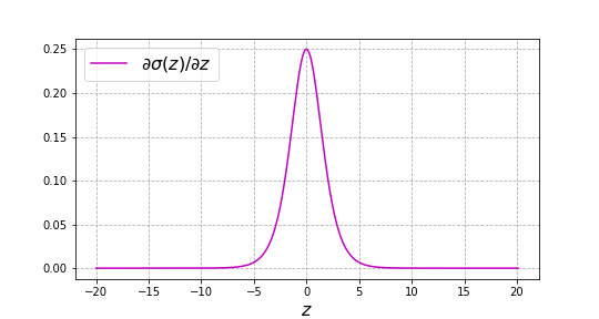
Plot of $\sigma'(z)$, the derivative of the sigmoid function $\sigma(z)$.

According to Eq. (\ref{derivative}), we can write

We will later come back to Eq. (\ref{logitSigma}), (\ref{derivative1}) and (\ref{derivative2}).

A model to estimate probabilities

To classify any sample $\mathbf{x}$, assuming a probabilistic model, we are interested in estimating $P(y = 1 \;\vert\; \mathbf{x})$ and $P(y = 0 \;\vert\; \mathbf{x})$. To minimize the classification error, according to Bayesian decision theory, we should classify samples as follows

In practice, since $P(y = 1 \;\vert\; \mathbf{x}) + P(y = 0 \;\vert\; \mathbf{x}) = 1$, one probability can be expressed as a function of the other one, and thus we only need to estimate one of them.

Logistic regression proposes using a sigmoid function $\sigma(z)$ to estimate $P\left(y = 1 \;\vert\; \mathbf{x}\right)$ and thus Eq. (\ref{ClassificationRuleBayes}) becomes

Since $\sigma(z)$ equals $0.5$ only when $z$ is null, then we can re-write the last condition as

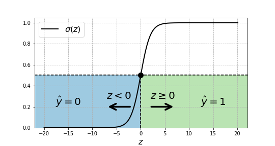
Decision regions and boundary. If $z \geq 0$ we decide $\hat{y}=1$, and $\hat{y}=0$ otherwise.

So far, we have a way to estimate $P(y = 1 \;\vert\; \mathbf{x})$ and a classification rule to label samples, yet, we still miss a definition for $z$. A priori, the guess is that the features that we have chosen are meaningful for the classification task, and thus that the variable $z$ should depend on them.

Defining parameters to adjust the estimations

For a sample $\mathbf{x}$, the product between $\mathbf{x}$ and a weighting vector $\mathbf{w} \in \mathbb{R}^N$ plus a bias or intercept $b \in \mathbb{R}$ determines the value that $z$ takes.

where to emphasize all variables on which $\hat{P}\left(y = 1 \;\vert\; \mathbf{x}\right)$ depends on, we rather use the notation $\hat{p_1}(\mathbf{x}, \mathbf{w}, b)$.

In Eq. (\ref{logitSigma}), replacing $\sigma(z)$ and $z$ respectively by $\hat{p_1}(\mathbf{x}, \mathbf{w}, b)$ and $\mathbf{w}^\intercal \mathbf{x} + b$, then we have

where the left term is known as the log-odds or logit of $\hat{p_1}(\mathbf{x}, \mathbf{w}, b)$. Hence, this means that the sigmoid function translates logits into probabilities.

Eq. (\ref{logitProba}) resembles the one we previously saw for linear regression, where $\hat{y} = \mathbf{w}^\intercal \mathbf{x} + b$. This gives us a hint of from where the name logistic regression comes from: we are applying a regression to the logits of $\hat{p_1}(\mathbf{x}, \mathbf{w}, b)$.

Classification Rule and Decision Boundary

Considering that $z = \mathbf{w}^\intercal \mathbf{x} + b$ in logistic regression, we can update the classification rule expressed in Eq. (\ref{ZDecisionBoundary}) as follows

Analyzing this expression, we can see that there exists a decision boundary in $\mathbf{w}^\intercal \mathbf{x} + b = 0$. The values of $\mathbf{x}$ that satisfy this condition form an (affine) hyperplane in the sub-space generated by $\left\{x_1, x_2, \ldots, x_n\right\}$, where $b$ is the quantity by which this hyperplane is shifted from the origin. When $\mathbf{w}$ and $b$ are known, if $\mathbf{x}$ is such that the computation of $\mathbf{w}^\intercal \mathbf{x} + b$ is greater than $0$, then $\hat{y} = 1$, and $\hat{y} = 0$ otherwise.

To better understand the effect of the different values that $\mathbf{w}$ and $b$ mat take, we can plot the sigmoid function against $\mathbf{x}$ instead of $z$, as we previously did.

We first focus on a case such that $N=1$. In these scenarios, $\mathbf{x}$ and $\mathbf{w}$ are, similar to $b$, scalars and thus respectively denoted $x$ and $w$. In the figure below, for a fixed value of $b$, from left to right, the plots reveal that the larger $w$ is, the sharper the S-shape of the sigmoid function becomes. In other words, $w$ allows to tune the steepness of the resulting function. On the other hand, keeping $w$ constant, we can see that modifying $b$ only shifts the position where the transition from $0$ to $1$ begins, i.e. the exact location where the threshold of 0.5 occurs changes, but the intrinsic shape of curve does not. Focusing on the decision boundaries, we can see that all sigmoid functions reach 0.5 when $x$ equals $-b/w$. Hence, for a fixed $w$, the influence of $b$ is larger the smaller $w$ is. For the samples such that $x < -b/w$, we have $\hat{y} = 0$, and for the remaining ones $\hat{y} = 1$.

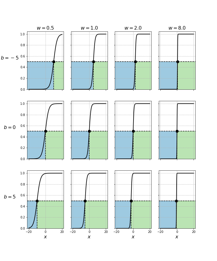
Decision regions and boundary for different values of $w$ and $b$ as function of $x$ when $N=1$.

On the other hand, when $N=2$, we have a sigmoid function of the type $\sigma(x_1 w_1 + x_2 w_2 + b)$. As before, the figure below reveals that increasing values of $w_1$ and $w_2$ lead to shaper transitions from $0$ to $1$, and changing the value of $b$ simply allows to place the 3D sigmoid function in different locations. Complementary to the 1-dimensional case, we see that the ratio $w_1/w_2$ allows to tune the rotation of the sigmoid surface. The decision boundary lies in $x_2 = -x_1 w_1 / w_2 - b/w_2$ for all cases, and can be more clearly seen on the left panels.

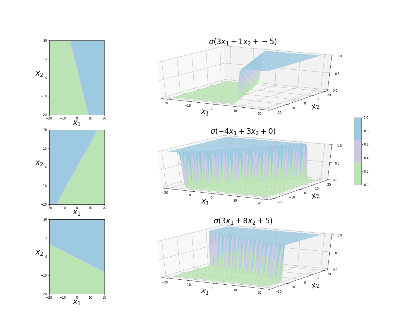
Decision regions and boundary as function of $x_1$ and $x_2$ when $N = 2$.

The same ideas hold on scenarios where $N > 2$, despite we cannot produce plots with the same level of details.

The question that remains at this point is how to choose the values of $\mathbf{w}$ and $b$.

Cross-Entropy Loss Function

The optimal values of $\mathbf{w}$ and $b$ can be estimated relying on the maximum likelihood estimation method. Given a training set $X$ of $m$ labeled i.i.d. samples, i.e. $X = \left\{(\mathbf{x}^{(1)}, y^{(1)}), (\mathbf{x}^{(2)}, y^{(2)}), \ldots, (\mathbf{x}^{(m)}, y^{(m)})\right\}$ , modelling $y$ as a Bernoulli variable with parameter $p(\mathbf{x})$, then the joint distribution for the dataset is

where $p(\mathbf{x}^{(i)})$ is the probability that sample $\mathbf{x}^{(i)}$ might belong to class $1$ and $y^{(i)}$ is the class to which $\mathbf{x}^{(i)}$ actually belongs to.

The log-likelihood, that we seek to maximize, can then be written as

Recalling that we estimate $p(\mathbf{x}^{(i)})$ as $\hat{p}_1(\mathbf{x}^{(i)}, \mathbf{w}, b) = \sigma(\mathbf{w}^\intercal \mathbf{x} + b)$, and defining the cost function $J(X, \mathbf{w}, b)$ as the negative version of the log-likelihood averaged over the $m$ samples composing the dataset, then

Since this mathematical expression resembles the one used in information theory to obtain the “cross-entropy” between two probability distributions, then this cost function is usually referred to as the cross-entropy loss function. An important, and convenient, characteristic of this function is that it is convex, i.e., it has a unique, and thus absolute, minimum.

Interpreting the Loss Function

Despite the cost function $J(X, \mathbf{w}, b)$ looks intricate, by further developing its expression, we can find a very intuitive way to understand it. For this, we need to note that, for any index $i$, $y^{(i)}$ can only evaluate to $1$ or $0$. Therefore, for each sample $(\mathbf{x}^{(i)}, y^{(i)})$, only one term out of the two addends in $J(X, \mathbf{w}, b)$ contributes to the cost function. We can use this fact to compress the expression of $J(X, \mathbf{w}, b)$ as follows

The figure below shows the functions that compose $c\left( y^{(i)}, \hat{p_1}(\mathbf{x}^{(i)}, \mathbf{w}, b)\right)$. For example, when $y^{(i)} = 1$, if $\hat{p_1}(\mathbf{x}^{(i)}, \mathbf{w}, b) = 1$, then the cost contributed by sample $(\mathbf{x}^{(i)}, y^{(i)})$ is 0. However, on the opposite extreme, if $\hat{p_1}(\mathbf{x}^{(i)}, \mathbf{w}, b) = 0$, then the cost would become infinite. For intermediate values, the logarithm in the expression leads to penalize more “worse” decisions, e.g., for $y^{(i)} = 1$, the smaller $\hat{p_1}(\mathbf{x}^{(i)}, \mathbf{w}, b)$ is, the much larger $\log\left(\hat{p_1}(\mathbf{x}^{(i)}, \mathbf{w}, b)\right)$ will be. In addition, analyzing the cost for $y^{(i)} = 0$, we can see that it is a shifted mirrored copy of that for $y^{(i)} = 1$: the curve is identical, but rather penalizing more severely the more that $\hat{p_1}(\mathbf{x}^{(i)}, \mathbf{w}, b)$ is closer to $1$.

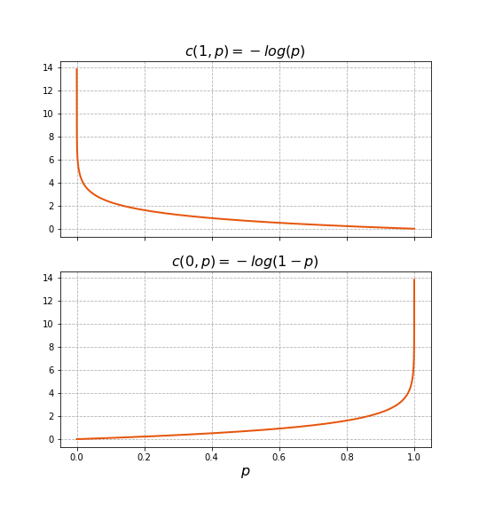
Cost function composition.

Finally, it must be noted that, even if our classifier would have made correct classifications, e.g. estimated $\hat{p_1}(\mathbf{x}^{(i)}, \mathbf{w}, b) > 0.5$ in a case where $y^{(i)} = 1$, we are still increasing the cost function by $c\left( y^{(i)}, \hat{p_1}(\mathbf{x}^{(i)}, \mathbf{w}, b)\right)$. Indeed, the cost function does not penalize classification mistakes, but more generally the fact that the classifier makes “doubtful” classifications. In other words, for all samples where the classifier was not completely “convinced” or “sure” of its choice, $J(X, \mathbf{w}, b)$ increases. In particular, using the cross-entropy loss function as the cost function tends to generate estimations that, for all samples, resemble as closely as possible the real values of $y$.

When the true distributions of $y=1 \;\vert\; \mathbf{x}$ and $y=0 \;\vert\; \mathbf{x}$ are clearly distinguishable, we would want our classifier not to hesitate. This means that, for all samples $\mathbf{x}^{(i)}$ and $\mathbf{x}^{(j)}$ in our training set for which $y^{(i)}=1$ and $y^{(j)}=0$ we would like to end up computing $\hat{p_1}(\mathbf{x}^{(i)}, \mathbf{w}, b) = 1$ and $\hat{p_1}(\mathbf{x}^{(i)}, \mathbf{w}, b) = 0$, respectively. On the other hand, when the true distributions overlap, our hope is that we will find values of $\mathbf{w}$ and $b$ such that the estimations will be confident for most training samples. However, for those samples close to the decision boundary, we expect to see that our classifier is less confident. In an attempt to improve the estimation on these samples, we may try to further tune $\mathbf{w}$ and $b$. However, it is likely that improving the estimation on one sample makes worse the one obtained for another sample. All in all, the best values for $\mathbf{w}$ and $b$ are those for which the estimations have a high confidence for most samples, and also balance well the aforementioned trade-off.

Optimizing the parameters

To find the optimal value of $\mathbf{w}$ and $b$, we need to minimize the cost function $J(X, \mathbf{w}, b)$. Analyzing Eq. (\ref{cost-function}), we can see that $J(X, \mathbf{w}, b)$ is a composition of differentiable functions, and thus is differentiable itself. This means that we can find the minimum of $J(X, \mathbf{w}, b)$ looking for the point where all the partial derivatives become null.

To begin, we can first focus on the derivative of $J(X, \mathbf{w}, b)$ with respect to component $w_j$ of $\mathbf{w}$. Noting that in Eq. (\ref{cost-function}), $y^{(i)}$ does not depend on $w_j$, then we only need to find the derivatives of $\log\left(\left. \sigma(z) \right\rvert_{z = \mathbf{w}^\intercal \mathbf{x} + b}\right)$ and $\log\left(1 - \left. \sigma(z) \right\rvert_{z = \mathbf{w}^\intercal \mathbf{x} + b}\right)$.

To derive these calculations, first note that

where it is trivial to see that $\frac{\partial z}{\partial w_j} = x_j^{(i)}$. Hence, we only need to find $\frac{\partial J(X, \mathbf{w}, b)}{\partial z}$. In particular, since

we can use the results of Eq. (\ref{derivative1}) and (\ref{derivative2}) to solve each of these calculations. We can proceed in a similar way to find the derivative with respect to $b$, just noticing that $\frac{\partial z}{\partial b} = 1$. By further applying some algebra, it is simple to show that

Eq. (\ref{dJdw-LR}) and (\ref{dJdb-LR}) can be conveniently expressed in a vectorized way, relying on matrix notation

Unfortunately, setting these equations to zero results into what are called transcendental equations, i.e., equations for which there is no closed form to solve them. To overcome this limitation, the only option left is to rely on numerical solutions e.g. the gradient descent algorithm. Regardless of the optimization algorithm that is chosen, since $J(X, \mathbf{w}, b)$ is convex, converging towards the only, and thus optimal, minimum is ensured provided that multiple iterations are performed.

During the training, the values of $\mathbf{w}$ and $b$ will be iteratively updated, hence modifying the positioning of the hyperplane that serves as decision boundary for the classification problem. Hopefully, at the end of the process, the hyperplane will end up “well” located, i.e., for most training samples, the estimations and classifications the algorithm performs will be reasonably good. An example can be seen below.

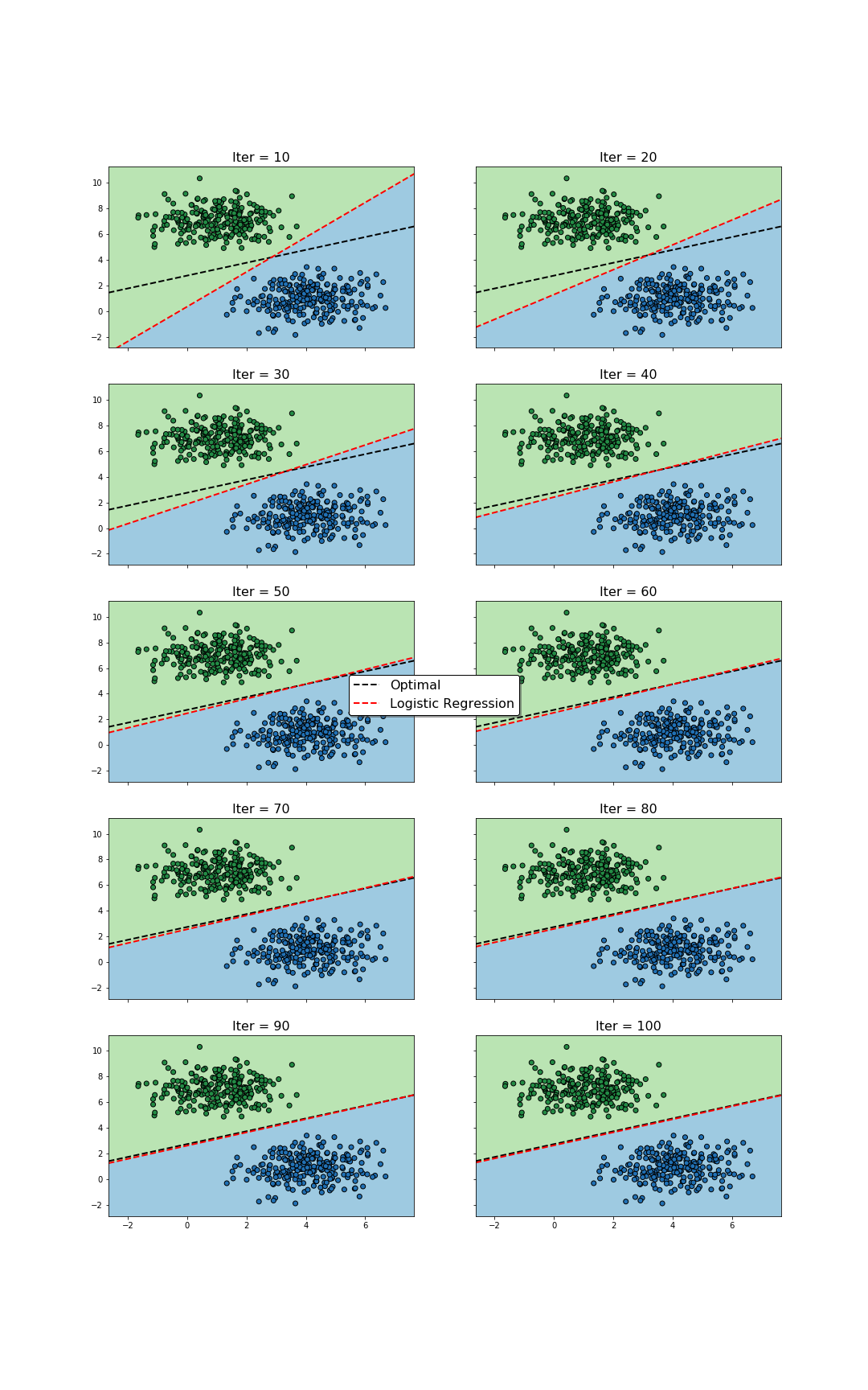
Update of decision regions during the training process. The values of $\mathbf{w}$ and $b$ change as the optimization algorithm is run. As a consequence, for different number of iterations, different decision boundaries are found. Towards the beginning, the changes are visually larger, contrasting with the end of the process, where the boundary does not change much. The optimal decision boundary serves as reference, and is only known since the data was synthetically generated.

A complementary view, highlighting the changes in the decision boundary for larger number of iterations, is shown below.

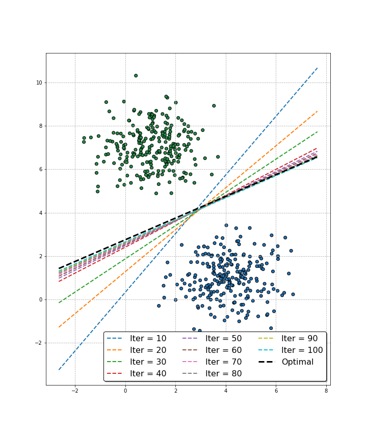
Decision boundary as a function of the number of iterations. We can see that despite the changes towards the end of the training process seem negligible, the algorithm is still able to better approach the optimal decision boundary.

Finally, the figure below shows the 3D sigmoid function resulting at the end of the decision process. In addition, the plot includes the training samples where the z-axis represents the corresponding label for each of them.

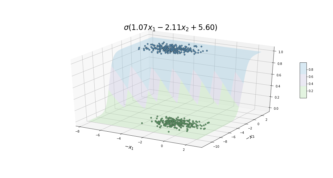
Fitted 3D sigmoid function.

Logistic Regression in Action

We have analyzed logistic regression in detail; now it is time to see how it performs on different examples.

First, we could wonder what happens when we have representative datasets for the same classification problem. If instead of aggregating them, we run logistic regression in each of these datasets, we expect to see that the estimated decision boundary changes at each time. However, all decision boundaries will be found to fluctuate around the optimal decision boundary. This can be seen in the figure below.

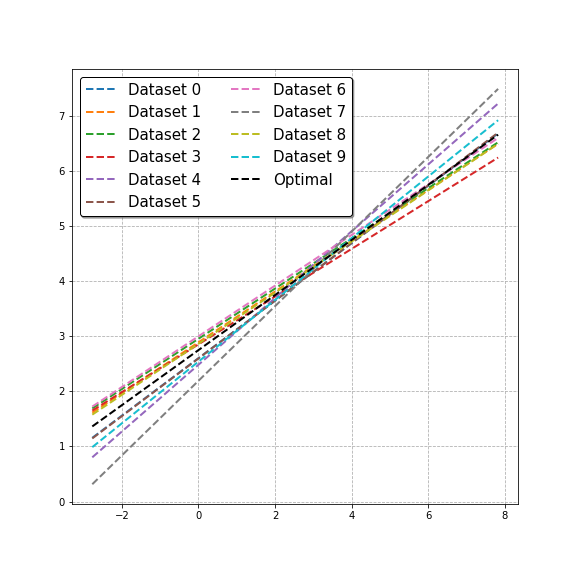
Logistic regression applied to representative training sets of different classification problems.

On the other hand, given training sets of different problems, the image below shows the decision boundaries that logistic regression finds for each case. As we can see, the performance for each problem is rather reasonable.

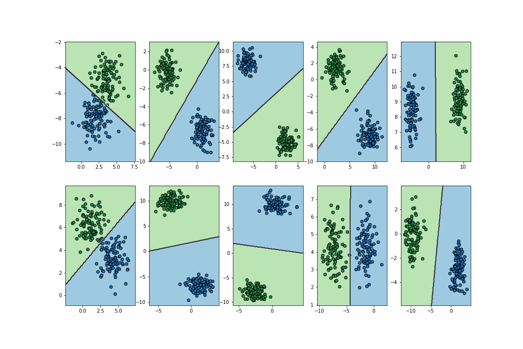
Logistic regression applied to representative training sets of different classification problems.

Finally, it is important to mention that we can also obtain non-linear decision boundaries relying on logistic regression. For this to be possible, polynomial and interaction terms among the different features need to be used. As a rule of thumb, a good approach is to set the largest polynomial order to a “high” value, e.g. 4 or 5, and apply regularization to avoid over-fitting. In addition, standardizing the features may help the algorithm to converge. An example of the performance of logistic regression in cases like this can be seen below.

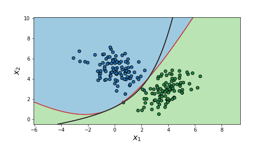
Estimated (red) and optimal (black) non-linear decision boundaries.

Multinomial Classification

A logistic regression classifier only works for binary classification problems. However, multiple of these classifiers can be used to handle cases where $y$ may take more than two values, i.e., $K>2$. In particular, two different approaches exist to combine binary classifiers: one-vs-the-rest (OvR), also called one-vs-all (OvA), and one-vs-one (OvO).

While workarounds such as OvR/OvA and OvO allow to use logistic regression for multinomial classification tasks, softmax regression is a method specifically conceived for this purpose. In addition, linear and quadratic discriminant analysis, and also K-nearest-neighbours, can be used instead.