Lagrange Interpolation

I sometimes need a function, and want it to be both weird and sexy. To define this function, I want to be unstructured, I don’t want to limit my imagination. I want to be able to define a set of ordered points, and then have a function that when plotted, its graph passes through them. But I need more than just being able to plot the function, I need to know its exact expression, so that I can use it later. Can we do that? That is, can we find a closed form to express such a function?

And as Obama would have said many years ago, yes we can! Given $n + 1$ points, there exists a polynomial of degree $n$ that meets this condition. Not that I particularly wanted a polynomial, but I can settle with that. The idea sounds more sexy the moment you are told that there is a unique polynomial of degree $n$ complying with such constraints.

Do you want to find it? I want. Let’s go!

A polynomial, what?

A polynomial of degree $n$ is a function $P (x)$ that can be written as

\begin{matrix} (1) & P (x) = \sum_{k = 0}^{n} a_{k} x^{k} = a_{0} + a_{1} x + a_{2} x^{2} + \dots + a_{n} x^{n} \end{matrix}

The set ${a_{0}, a_{1}, \dots, a_{n}}$ are the coefficients of the polynomial. As the values of these coefficients change, we obtain a different polynomial each time.

Polynomials of $x$ .

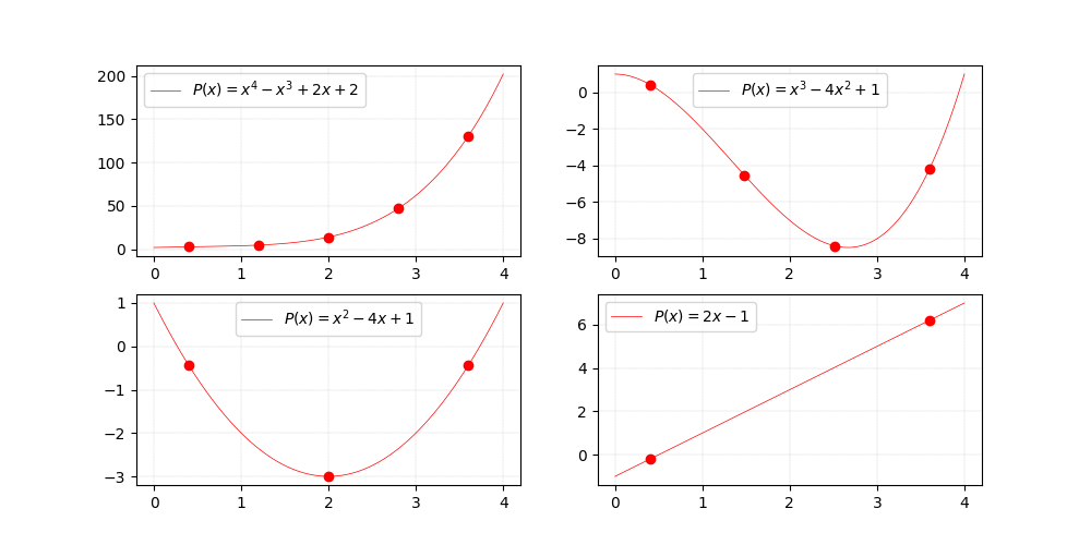
If we plot $P (x)$ , the exact shape of the curve we obtain depends on the coefficients of the polynomial, as shown on the figure on top.

A system of equations

Our problem is finding the coefficients’ values for which the graph of $P (x)$ indeed traverses the requested $n + 1$ points.

And what can we do to find them? Well, the points need to be in the image of $P (x)$ . That is, for each point $(x_{j}, y_{j})$ in the set, we know that $P (x_{j}) = y_{j}$ must hold. As we have $n + 1$ points, evaluating $P (x)$ , we can create a system of $n + 1$ equations.

\begin{aligned} (2) & P (x_{0}) & = a_{0} + a_{1} x_{0} + a_{2} x_{0}^{2} + \dots + a_{n} x_{0}^{n} = y_{0} \\ (3) & P (x_{1}) & = a_{0} + a_{1} x_{1} + a_{2} x_{1}^{2} + \dots + a_{n} x_{1}^{n} = y_{1} \\ ⋮ \\ (4) & P (x_{n}) & = a_{0} + a_{1} x_{n} + a_{2} x_{n}^{2} + \dots + a_{n} x_{n}^{n} = y_{n} \end{aligned}

To find the answer to our problem, we need to solve the system.

Things look good a priori, as in general we can only find the values of $n + 1$ unknowns (the coefficients) if we have the same number of equations.

Bring on the matrices

We switch to matrix notation and define

\begin{matrix} (5) & X = [\begin{matrix} 1 & x_{0} & \dots & x_{0}^{n} \\ 1 & x_{1} & \dots & x_{1}^{n} \\ ⋮ & ⋮ & ⋮ \\ 1 & x_{n} & \dots & x_{n}^{n} \end{matrix}] a = [\begin{matrix} a_{0} \\ a_{1} \\ ⋮ \\ a_{n} \end{matrix}] y = [\begin{matrix} y_{0} \\ y_{1} \\ ⋮ \\ y_{n} \end{matrix}] \end{matrix}

so that then we can describe our problem more compactly as

\begin{matrix} (6) & X \cdot a = y \end{matrix}

In particular, $X \in R^{(n + 1) \times (n + 1)}$ is not just any other square matrix, it is actually known as the the Vandermonde matrix.

A solution, but not THE solution

Thanks to good old Algebra, after switching the notation, we see that in the end, the solution is to simply get

\begin{matrix} (7) & a = X^{- 1} \cdot y \end{matrix}

End of story? Well…just hold on to your belts!

First, we should ask ourselves whether $X^{- 1}$ even exists. As $X$ is a square matrix, it could indeed be the case. In fact, I am sure there is a proof for this, but just looking at the expression, you can already tell that the inverse of this matrix exists as long as $\forall j \neq k, x_{j} \neq x_{k}$ . That is, there should not be two points requesting some image for the same domain value. Say we had $(x_{p}, y_{a})$ and $(x_{p}, y_{b})$ in our set of points. If $y_{a} \neq y_{b}$ , then the problem would be messed up from scratch: a well-defined function can only have a unique image per domain element. If instead $y_{a} = y_{b}$ , then we would have a point that repeats in our set, and we would only have be able to construct $n$ linearly independent equations. In this case, rather than a unique polynomial of degree $n$ , the solution would consist of a sub-space of polynomials.

Second, to compute $X^{- 1}$ , how much computational power do we need? Again without proof, but without doubts neither, I’m sorry to break it to you, me, and everyone else, but computing this matrix is an $O (n^{3})$ operation…so as soon as $n$ becomes of a moderate value, good luck waiting for that to run!

Fortunately, Lagrange came to the rescue and saved us all.

Lagrange Interpolation

Lagrange changed a little bit the way we were thinking about the problem, and proposed to think the polynomial $P (x)$ as the sum of $n + 1$ functions

\begin{matrix} (8) & P (x) = \sum_{i = 0}^{n} α_{i} ϕ_{i} (x) = α_{0} ϕ_{0} (x) + α_{1} ϕ_{1} (x) + \dots + α_{n} ϕ_{n} (x) \end{matrix}

and then proved that the solution was to define

\begin{matrix} (9) & α_{i} = y_{i} \end{matrix}

\begin{matrix} (10) & ϕ_{i} (x) = \frac{\prod_{j \neq i} x - x_{j}}{\prod_{j \neq i} x_{i} - x_{j}} \end{matrix}

Analyzing the expressions, we see that $\forall j \neq i, ϕ_{i} (x_{j}) = 0$ . In addition, $ϕ_{i} (x_{i}) = 1$ and as $α_{i} = y_{i}$ , then $α_{i} ϕ_{i} (x_{i}) = y_{i}$ . This way, for each point $(x_{k}, y_{k})$ , out of all the functions composing $P (x)$ , there is only $α_{k} ϕ_{k} (x)$ that evaluated at $x_{k}$ returns $y_{k}$ , while the other $n$ functions are nil.

I mean…what a beast, such a clever and elegant solution. Chapeau!

The interpolation in action

Let’s analyse one case to convince ourselves! Say we want a function for the following $5$ points.

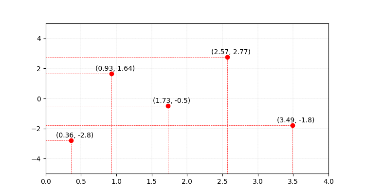
Points that must be on the image of $P (x)$ .

I guess we would all panic if we are asked to solve this, but we just learned about Lagrange’s interpolation, so we know we can find the polynomial of degree $4$ that meets this condition.

In particular, let’s gather the functions that compose $P (x)$ :

xx = np.linspace(0, 4, 200)

a1phi1 = -2.8 * \
    ((xx - 0.93) * (xx - 1.73) * (xx - 2.57) * (xx - 3.49)) / \
    ((0.36 - 0.93) * (0.36 - 1.73) * (0.36 - 2.57) * (0.36 - 3.49))

a2phi2 = 1.64 * \
    ((xx - 0.36) * (xx - 1.73) * (xx - 2.57) * (xx - 3.49)) / \
    ((0.93 - 0.36) * (0.93 - 1.73) * (0.93 - 2.57) * (0.93 - 3.49))

a3phi3 = -0.5 * \
    ((xx - 0.36) * (xx - 0.93) * (xx - 2.57) * (xx - 3.49)) / \
    ((1.73 - 0.36) * (1.73 - 0.93) * (1.73 - 2.57) * (1.73 - 3.49))

a4phi4 = 2.77 * \
    ((xx - 0.36) * (xx - 0.93) * (xx - 1.73) * (xx - 3.49)) / \
    ((2.57 - 0.36) * (2.57 - 0.93) * (2.57 - 1.73) * (2.57 - 3.49))

a5phi5 = -1.8 * \
    ((xx - 0.36) * (xx - 0.93) * (xx - 1.73) * (xx - 2.57)) / \
    ((3.49 - 0.36) * (3.49 - 0.93) * (3.49 - 1.73) * (3.49 - 2.57))

And let’s just plot and see how these functions look like.

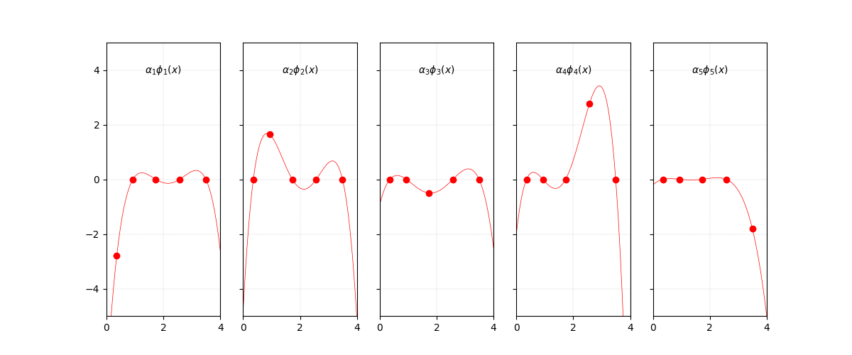
Functions that compose $P (x)$ .

The first feeling when you look at this is “oh, it will be hard to prove that this truly adds up to what we need”. But to simplify, recall that each function focuses on one point at a time, while ensuring it does not bother the other. This is why, for the points highlighted, there is only one where $y \neq 0$ and for the others $y = 0$ . Things are actually looking good then!

Final step, let’s add these functions and see what we get.

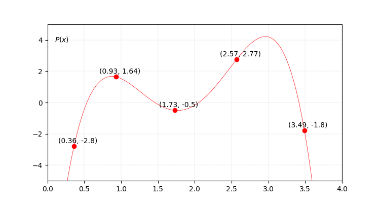
Resulting $P (x)$ .

An image sometimes is worth more than a million words, so I will limit myself to simpley say beautiful.

Generalizing: any and all polyomials?!

A natural question that follows is whether we could not have found a more “compact” solution that the one that Lagrange proposed. In short, the answer is no, but let’s reason about it. For example, if we were able to find some linear dependency among the $ϕ_{i} (x)$ functions, removing it we could maybe come up with another solution for $P (x)$ , composing it with less than $n + 1$ functions. Well, dreaming is ok, but if that is how we come up with solutions, Lagrange clearly had very sweet dreams long ago: his solution actually conforms a basis for the space of polynomials of degree $n$ (note that this space is of dimension $n + 1$ ).

The fact that the set of Lagrange’s functions $ϕ_{i} (x)$ conforms a basis means that, relying these functions:

we can produce all the polynomials of degree $n$ , and;
for each polynomial, there is a unique combination of the $ϕ_{i} (x)$ functions that produce them.

For example, another basis for the same sub-space is the canonical one, conformed by the functions ${1, x, x^{2} \dots, x^{n}}$ , as shown below for $n = 4$ .

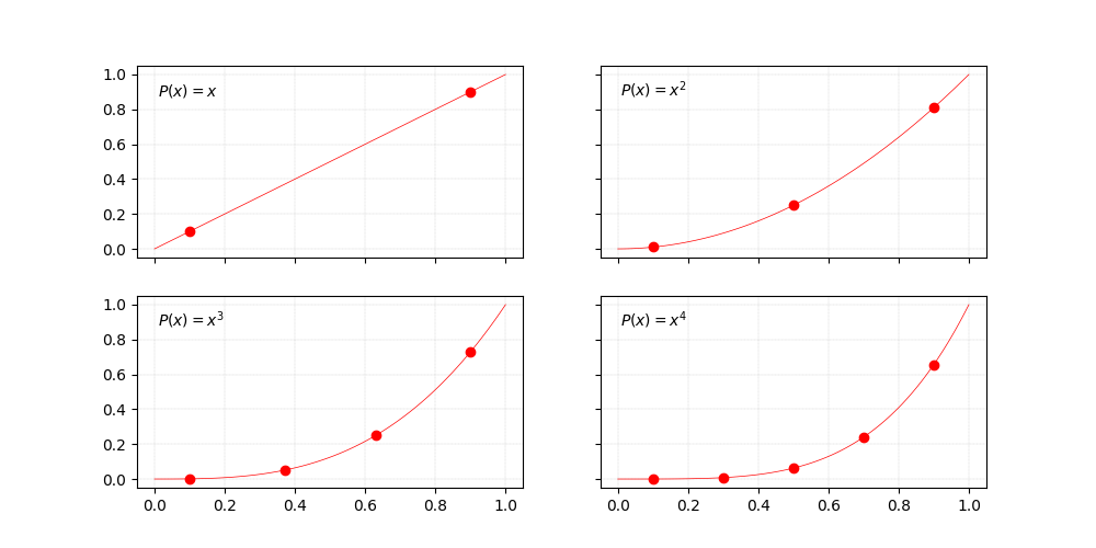
Polynomials of degree $n \geq 1$ for the canonical basis of degree $4$ .

I know, if we compare the functions on the plot we just obtained for the canonical basis with the ones from Lagrange’s interpolation we calculated before, it is human to hesitate …are we sure that the very clever formulation of Lagrange is also a basis? Well, only reason can defeat fear, so let’s prove it to convince ourselves.

To verify that Lagrange’s functions conform a basis of the $n$ -degree polynomials, we need to work with a linear combination these functions

\begin{matrix} (11) & L (x) = β_{0} ϕ_{0} (x) + β_{1} ϕ_{1} (x) + \dots + β_{n} ϕ_{n} (x) \end{matrix}

If we can show that $\forall x, L (x) = 0 \Leftrightarrow \forall i, β_{i} = 0$ , then it is true.

As the aforementioned condition must hold for all $x$ , then in particular it must hold for ${x_{0}, x_{1}, \dots, x_{n}}$ , the x-coordinates of the $n + 1$ points used to define the $ϕ_{i} (x)$ functions. Without loosing generality, taking $x_{0}$ as an example, we can compute

\begin{matrix} (12) & L (x_{0}) = β_{0} ϕ_{0} (x_{0}) + β_{1} ϕ_{1} (x_{0}) + \dots + β_{n} ϕ_{n} (x_{0}) = 0 \end{matrix}

but based on our previous analysis, we know that this ends up evaluating to $L (x_{0}) = β_{0} = 0$ . We can iterate over the $n$ remaining $x_{i}$ values following a similar procedure to prove that in each step $i$ , we need $β_{i} = 0$ to hold. And once this is done, we just need to prove the other direction of the implication, but the proof is trivial. Hence, voila, we have proved that Lagrange’s solution is indeed a basis of the $n$ polynomial space.

We need to agree that Lagrange’s solution is simply beautiful, isn’t it?

Implementing Lagrange’s interpolation

Now that we know many things about Lagrange’s interpolation, the last point I want to address is how to implement it efficiently in code. To reason about this, let’s first write down the final expression of $P (x)$ :

\begin{matrix} (13) & P (x) = \sum_{i = 0}^{n} y_{i} \frac{\prod_{j \neq i} x - x_{j}}{\prod_{j \neq i} x_{i} - x_{j}} \end{matrix}

And I will continue writing soon…